Queues and Congestion Management
Congestion management defines a policy that determines the order in which packets are forwarded and specifies drop principles for packets. The queuing technology is used.
The queuing technology orders packets in the buffer. When the packet rate exceeds the interface bandwidth or the bandwidth allocated to the queue that buffers packets, the packets are buffered in queues and wait to be forwarded. The queue scheduling algorithm determines the order in which packets are leaving a queue and the relationships between queues.

The Traffic Manager (TM) on the forwarding plane houses high-speed buffers, for which all interfaces have to compete. To prevent traffic interruptions due to long-time loss in the buffer battle, the system allocates a small buffer to each interface and ensures that each queue on each interface can use the buffer.
The TM puts received packets into the buffer and allows these packets to be forwarded in time when traffic is not congested. In this case, the period during which packets are stored in the buffer is at μs level, and the delay can be ignored.
When traffic is congested, packets accumulate in the buffer and wait to be forwarded. The delay greatly prolongs. The delay is determined by the buffer size for a queue and the output bandwidth allocated to a queue. The format is as follows:
Delay of a queue = Buffer size for the queue/Output bandwidth for the queue
The NetEngine 8000 F device allocates eight port queues to each interface. These eight port queues are also called class queues (CQs). The eight queues are BE, AF1, AF2, AF3, AF4, EF, CS6, and CS7. EF, CS6 and CS7 use PQ scheduling by default, BE, AF1, AF2, AF3 and AF4 use WFQ scheduling. For details, see the Port Queue Scheduling.
The first in first out (FIFO) mechanism is used to transfer packets in a queue. Resources used to forward packets are allocated based on the arrival order of packets.
Scheduling Algorithms
The commonly used scheduling algorithms are as follows:
- First In First Out (FIFO)
- Strict Priority (SP)
- Round Robin (RR)
- Weighted Round Robin (WRR)
- Deficit Round Robin (DRR)
- Weighted Deficit Round Robin (WDRR)
- Weighted Fair Queuing (WFQ)
FIFO
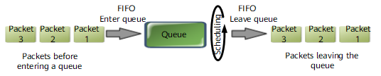
FIFO does not need traffic classification. As shown in Figure 1, FIFO allows the packets that come earlier to enter the queue first. On the exit of a queue, FIFO allows the packets to leave the queue in the same order as that in which the packets enter the queue.
SP
SP schedules packets strictly based on queue priorities. Packets in queues with a low priority can be scheduled only after all packets in queues with a high priority have been scheduled.
As shown in Figure 2, three queues with a high, medium, and low priority respectively are configured with SP scheduling. The number indicates the order in which packets arrive.

When packets leave queues, the device forwards the packets in the descending order of priorities. Packets in the higher-priority queue are forwarded preferentially. If packets in the higher-priority queue come in between packets in the lower-priority queue that is being scheduled, the packets in the high-priority queue are still scheduled preferentially. This implementation ensures that packets in the higher-priority queue are always forwarded preferentially. As long as there are packets in the high queue no other queue will be served. If all packets have only one priority, the FIFO principle is used to forward packets.
The disadvantage of SP is that the packets in lower-priority queues are not processed until all the higher-priority queues are empty. As a result, a congested higher-priority queue causes all lower-priority queues to starve.
RR
RR schedules multiple queues in ring mode. If the queue on which RR is performed is not empty, the scheduler takes one packet away from the queue. If the queue is empty, the queue is skipped, and the scheduler does not wait.

WRR
Compared with RR, WRR can set the weights of queues. During the WRR scheduling, the scheduling chance obtained by a queue is in direct proportion to the weight of the queue. RR scheduling functions the same as WRR scheduling in which each queue has a weight 1.
WRR configures a counter for each queue and initializes the counter based on the weight values. Each time a queue is scheduled, a packet is taken away from the queue and being transmitted, and the counter decreases by 1. When the counter becomes 0, the device stops scheduling the queue and starts to schedule other queues with a non-0 counter. When the counters of all queues become 0, all these counters are initialized again based on the weight, and a new round of WRR scheduling starts. In a round of WRR scheduling, the queues with the larger weights are scheduled more times.

In an example, three queues with the weight 50%, 25%, and 25% respectively are configured with WRR scheduling.
The counters are initialized first: Count[1] = 2, Count[2] = 1, and Count[3] = 1.
First round of WRR scheduling:
Packet 1 is taken from queue 1, with Count[1] = 1. Packet 5 is taken from queue 2, with Count[2] = 0. Packet 8 is taken from queue 3, with Count[3] = 0.
Second round of WRR scheduling:
Packet 2 is taken from queue 1, with Count[1] = 0. Queues 2 and 3 do not participate in this round of WRR scheduling since Count [2] = 0 and Count[3] = 0.
Then, Count[1] = 0; Count[2] = 0; Count[3] = 0. The counters are initialized again: Count[1] = 2; Count[2] = 1; Count[3] = 1.
Third round of WRR scheduling:
Packet 3 is taken from queue 1, with Count[1] = 1. Packet 6 is taken from queue 2, with Count[2] = 0. Packet 9 is taken from queue 3, with Count[3] = 0.
Fourth round of WRR scheduling:
Packet 4 is taken from queue 1, with Count[1] = 0. Queues 2 and 3 do not participate in this round of WRR scheduling since Count [2] = 0 and Count[3] = 0.
Then, Count[1] = 0; Count[2] = 0; Count[3] = 0. The counters are initialized again: Count[1] = 2; Count[2] = 1; Count[3] = 1.
In statistical terms, you can see that the times for the packets to be scheduled in each queue is in direct ratio to the weight of this queue. The higher the weight, the more the times of scheduling. If the interface bandwidth is 100 Mbit/s, the queue with the lowest weight can obtain a minimum bandwidth of 25 Mbit/s, preventing packets in the lower-priority queue from being starved out when SP scheduling is implemented.
During the WRR scheduling, the empty queue is directly skipped. Therefore, when the rate at which packets arrive at a queue is low, the remaining bandwidth of the queue is used by other queues based on a certain proportion.
WRR scheduling has two disadvantages:
- WRR schedules packets based on the number of packets. Therefore, each queue has no fixed bandwidth. With the same scheduling chance, a long packet obtains higher bandwidth than a short packet. Users are sensitive to the bandwidth. When the average lengths of the packets in the queues are the same or known, users can obtain expected bandwidth by configuring WRR weights of the queues; however, when the average packet length of the queues changes, users cannot obtain expected bandwidth by configuring WRR weights of the queues.
- Services that require a short delay cannot be scheduled in time.
DRR
The scheduling principle of DRR is similar to that of RR.
RR schedules packets based on the packet number, whereas DRR schedules packets based on the packet length.
DRR configures a counter Deficit for each queue. The counters are initialized as the maximum bytes (assuming Quantum, generally the MTU of the interface) allowed in a round of DRR scheduling. Each time a queue is scheduled, if the packet length is smaller than Deficit, a packet is taken away from the queue, and the Deficit counter decreases by 1. If the packet length is greater than Deficit, the packet is not sent, and the Deficit value remains unchanged. The system continues to schedule the next queue. After each round of scheduling, Quantum is added for each queue, and a new round of scheduling is started. Unlike SP scheduling, DRR scheduling prevents packets in low-priority queues from being starved out. However, DRR scheduling cannot set weights of queues and cannot schedule services requiring a low-delay (such as voice services) in time.
MDRR
Modified Deficit Round Robin (MDRR) is an improved DRR algorithm. MDRR and DRR implementations are similar. MDRR allows the Deficit to be a negative so that long packets can be properly scheduled. In the next round of scheduling, however, this queue will not be scheduled. When the counter becomes 0 or a negative, the device stops scheduling the queue and starts to schedule other queues with a positive counter.
In an example, the MTU of an interface is 150 bytes. Two queues Q1 and Q2 use MDRR scheduling. Multiple 200-byte packets are buffered in Q1, and multiple 100-byte packets are buffered in Q2. Figure 5 shows how DRR schedules packets in these two queues.

As shown in Figure 5, after six rounds of MDRR scheduling, three 200-byte packets in Q1 and six 100-byte packets in Q2 are scheduled. The output bandwidth ratio of Q1 to Q2 is actually 1:1.
MDRR is an improved DRR algorithm. MDRR and DRR implementations are similar. Unlike MDRR, DRR allows the Deficit to be a negative so that long packets can be properly scheduled. In the next round of scheduling, however, this queue will not be scheduled. When the counter becomes 0 or a negative, the device stops scheduling the queue and starts to schedule other queues with a positive counter.
WDRR
Compared with DRR, Weighted Deficit Round Robin (WDRR) can set the weights of queues. DRR scheduling functions the same as WDRR scheduling in which each queue has a weight 1.
WDRR configures a counter, which implies the number of excess bytes over the threshold (deficit) in the previous round for each queue. The counters are initialized as the Weight x MTU. Each time a queue is scheduled, a packet is taken away from the queue, and the counter decreases by 1. When the counter becomes 0, the device stops scheduling the queue and starts to schedule other queues with a non-0 counter. When the counters of all queues become 0, all these counters are initialized as weight x MTU, and a new round of WDRR scheduling starts.
In an example, the MTU of an interface is 150 bytes. Two queues Q1 and Q2 use DRR scheduling. Multiple 200-byte packets are buffered in Q1, and multiple 100-byte packets are buffered in Q2. The weight ratio of Q1 to Q2 is 2:1. Figure 6 shows how WDRR schedules packets.
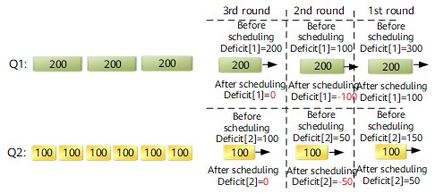
First round of WDRR scheduling:
The counters are initialized as follows: Deficit[1] = weight1 x MTU = 300 and Deficit[2] = weight2 x MTU=150. A 200-byte packet is taken from Q1, and a 100-byte packet is taken from Q2. Then, Deficit[1] = 100 and Deficit[2] = 50.
Second round of WDRR scheduling:
A 200-byte packet is taken from Q1, and a 100-byte packet is taken from Q2. Then, Deficit[1] = -100 and Deficit[2] = -50.
Third round of WDRR scheduling:
The counters of both queues are negatives. Therefore, Deficit[1] = Deficit[1] + weight1 x MTU = -100 + 2 x 150 = 200 and Deficit[2] = Deficit[2] + weight2 x MTU = -50 + 1 x 150 = 100.
A 200-byte packet is taken from Q1, and a 100-byte packet is taken from Q2. Then, Deficit[1] = 0 and Deficit[2] = 0.
As shown in Figure 6, after three rounds of WDRR scheduling, three 200-byte packets in Q1 and three 100-byte packets in Q2 are scheduled. The output bandwidth ratio of Q1 to Q2 is actually 2:1, which conforms to the weight ratio.
WDRR scheduling prevents packets in low-priority queues from being starved out and allows bandwidths to be allocated to packets based on the weight ratio when the lengths of packets in different queues vary or change greatly.
However, WDRR scheduling does not schedule services requiring a low-delay (such as voice services) in time.
WFQ
WFQ allocates bandwidths to flows based on the weight. In addition, to allocate bandwidths fairly to flows, WFQ schedules packets in bits. Figure 7 shows how bit-by-bit scheduling works.

The bit-by-bit scheduling mode shown in Figure 7 allows the device to allocate bandwidths to flows based on the weight. This prevents long packets from preempting bandwidths of short packets and reduces the delay and jitter when both short and long packets wait to be forwarded.
The bit-by-bit scheduling mode, however, is an ideal one. A NetEngine 8000 Fperforms the WFQ scheduling based on a certain granularity, such as 256 B and 1 KB. Different boards support different granularities.
Advantages of WFQ:
- Different queues obtain the scheduling chances fairly, balancing delays of flows.
- Short and long packets obtain the scheduling chances fairly. If both short and long packets wait in queues to be forwarded, short packets are scheduled preferentially, reducing jitters of flows.
- The lower the weight of a flow is, the lower the bandwidth the flow obtains.
Port Queue Scheduling
You can configure SP scheduling or weight-based scheduling for eight queues on each interface of a NetEngine 8000 F. Eight queues can be classified into three groups, priority queuing (PQ) queues, WFQ queues, and low priority queuing (LPQ) queues, based on scheduling algorithms.
-
SP scheduling applies to PQ queues. Packets in high-priority queues are scheduled preferentially. Therefore, services that are sensitive to delays (such as VoIP) can be configured with high priorities.
In PQ queues, however, if the bandwidth of high-priority packets is not restricted, low-priority packets cannot obtain bandwidth and are starved out.
Configuring eight queues on an interface to be PQ queues is allowed but not recommended. Generally, services that are sensitive to delays are put into PQ queues.
-
Weight-based scheduling, such as WRR, WDRR, and WFQ, applies to WFQ queues.
-
LPQ queue is implemented on a high-speed interface (such as an Ethernet interface).
SP scheduling applies to LPQ queues. The difference is that when congestion occurs, the PQ queue can preempt the bandwidth of the WFQ queue whereas the LPQ queue cannot. After packets in the PQ and WFQ queues are all scheduled, the remaining bandwidth can be assigned to packets in the LPQ queue.
In the actual application, best effort (BE) flows can be put into the LPQ queue. When the network is overloaded, BE flows can be limited so that other services can be processed preferentially.
WFQ, PQ, and LPQ can be used separately or jointly for eight queues on an interface.
Scheduling Order
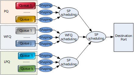
SP scheduling is implemented between PQ, WFQ, and LPQ queues. PQ queues are scheduled preferentially, and then WFQ queues and LPQ queues are scheduled in sequence, as shown in Figure 8. Figure 9 shows the detailed process.
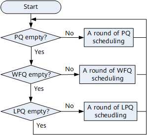
- Packets in PQ queues are preferentially scheduled, and packets in WFQ queues are scheduled only when no packets are buffered in PQ queues.
- When all PQ queues are empty, WFQ queues start to be scheduled. If packets are added to PQ queues afterward, packets in PQ queues are still scheduled preferentially.
- Packets in LPQ queues start to be scheduled only after all PQ and WFQ queues are empty.
Bandwidths are preferentially allocated to PQ queues to guarantee the peak information rate (PIR) of packets in PQ queues. The remaining bandwidth is allocated to WFQ queues based on the weight. If the bandwidth is not fully used, the remaining bandwidth is allocated to WFQ queues whose PIRs are higher than the obtained bandwidth until the PIRs of all WFQ queues are guaranteed. If any bandwidth is remaining at this time, the bandwidth resources are allocated to LPQ queues.
Bandwidth Allocation Example 1
In this example, the traffic shaping rate is set to 100 Mbit/s on an interface (by default, the traffic shaping rate is the interface bandwidth). The input bandwidth and PIR of each service are configured as follows.
Service Class |
Scheduling Mode |
Input Bandwidth (bit/s) |
PIR (bit/s) |
|---|---|---|---|
CS7 |
PQ |
65 M |
55 M |
CS6 |
PQ |
30 M |
30 M |
EF |
WFQ with the weight 5 |
10 M |
5 M |
AF4 |
WFQ with the weight 4 |
10 M |
10 M |
AF3 |
WFQ with the weight 3 |
10 M |
15 M |
AF2 |
WFQ with the weight 2 |
20 M |
25 M |
AF1 |
WFQ with the weight 1 |
20 M |
20 M |
BE |
LPQ |
100 M |
Not configured |
The bandwidth is allocated as follows:
- PQ scheduling is performed first. The 100 Mbit/s bandwidth is allocated to the CS7 queue first. The output bandwidth of CS7 equals the minimum rate of the traffic shaping rate (100 Mbit/s), input bandwidth of CS7 (65 Mbit/s), and PIR of CS7 (55 Mbit/s), that is, 55 Mbit/s. The remaining bandwidth 45 Mbit/s is allocated to the CS6 queue. The output bandwidth of CS6 equals the minimum rate of the traffic shaping rate (45 Mbit/s), input bandwidth of CS6 (30 Mbit/s), and PIR of CS6 (30 Mbit/s), that is, 30 Mbit/s. After PQ scheduling, the remaining bandwidth is 15 Mbit/s (100 Mbit/s - 55 Mbit/s - 30 Mbit/s).
- Then the first round of WFQ scheduling starts. The remaining bandwidth after PQ scheduling is allocated to WFQ queues. The bandwidth allocated to a WFQ queue is calculated based on this format: Bandwidth allocated to a WFQ queue = Remaining bandwidth x Weight of this queue/Sum of weights = 15 Mbit/s x Weight/15.
- Bandwidth allocated to the EF queue = 15 Mbit/s x 5/15 = 5 Mbit/s = PIR. The bandwidth allocated to the EF queue is fully used.
- Bandwidth allocated to the AF4 queue = 15 Mbit/s x 4/15 = 4 Mbit/s < PIR. The bandwidth allocated to the AF4 queue is exhausted.
- Bandwidth allocated to the AF3 queue = 15 Mbit/s x 3/15 = 3 Mbit/s < PIR. The bandwidth allocated to the AF3 queue is exhausted.
- Bandwidth allocated to the AF2 queue = 15 Mbit/s x 2/15 = 2 Mbit/s < PIR. The bandwidth allocated to the AF2 queue is exhausted.
- Bandwidth allocated to the AF1 queue = 15 Mbit/s x 1/15 = 1 Mbit/s < PIR. The bandwidth allocated to the AF1 queue is exhausted.
- The bandwidth is exhausted, and BE packets are not scheduled. The output BE bandwidth is 0.
The output bandwidth of each queue is configured as follows.
Service Class |
Scheduling Mode |
Input Bandwidth (bit/s) |
PIR (bit/s) |
Output Bandwidth (bit/s) |
|---|---|---|---|---|
CS7 |
PQ |
65 M |
55 M |
55 M |
CS6 |
PQ |
30 M |
30 M |
30 M |
EF |
WFQ with the weight 5 |
10 M |
5 M |
5 M |
AF4 |
WFQ with the weight 4 |
10 M |
10 M |
4 M |
AF3 |
WFQ with the weight 3 |
10 M |
15 M |
3 M |
AF2 |
WFQ with the weight 2 |
20 M |
25 M |
2 M |
AF1 |
WFQ with the weight 1 |
20 M |
20 M |
1 M |
BE |
LPQ |
100 M |
Not configured |
0 |
Bandwidth Allocation Example 2
In this example, the traffic shaping rate is set to 100 Mbit/s on an interface. The input bandwidth and PIR of each service are configured as follows.
Service Class |
Scheduling Mode |
Input Bandwidth (bit/s) |
PIR (bit/s) |
|---|---|---|---|
CS7 |
PQ |
15 M |
25 M |
CS6 |
PQ |
30 M |
10 M |
EF |
WFQ with the weight 5 |
90 M |
100 M |
AF4 |
WFQ with the weight 4 |
10 M |
10 M |
AF3 |
WFQ with the weight 3 |
10 M |
15 M |
AF2 |
WFQ with the weight 2 |
20 M |
25 M |
AF1 |
WFQ with the weight 1 |
20 M |
20 M |
BE |
LPQ |
100 M |
Not configured |
The bandwidth is allocated as follows:
- Packets in the PQ queue are scheduled preferentially to ensure the PIR of the PQ queue. After PQ scheduling, the remaining bandwidth is 75 Mbit/s (100 Mbit/s - 15 Mbit/s - 10 Mbit/s).
- Then the first round of WFQ scheduling starts. The remaining bandwidth after PQ scheduling is allocated to WFQ queues. The bandwidth allocated to a WFQ queue is calculated based on this format: Bandwidth allocated to a WFQ queue = Remaining bandwidth x Weight of this queue/Sum of weights = 75 Mbit/s x Weight/15.
- Bandwidth allocated to the EF queue = 75 Mbit/s x 5/15 = 25 Mbit/s < PIR. The bandwidth allocated to the EF queue is fully used.
- Bandwidth allocated to the AF4 queue = 75 Mbit/s x 4/15 = 20 Mbit/s > PIR. The AF4 queue actually obtains the bandwidth 10 Mbit/s (PIR). The remaining bandwidth is 10 Mbit/s.
- Bandwidth allocated to the AF3 queue = 75 Mbit/s x 3/15 = 15 Mbit/s = PIR. The AF3 queue actually obtains the bandwidth 10 Mbit/s (PIR). The remaining bandwidth is 5 Mbit/s.
- Bandwidth allocated to the AF2 queue = 75 Mbit/s x 2/15 = 10 Mbit/s < PIR. The bandwidth allocated to the AF2 queue is exhausted.
- Bandwidth allocated to the AF1 queue = 75 Mbit/s x 1/15 = 5 Mbit/s < PIR. The bandwidth allocated to the AF1 queue is exhausted.
- The remaining bandwidth is 15 Mbit/s, which is allocated to the queues, whose PIRs are higher than the obtained bandwidth, based on the weight.
- Bandwidth allocated to the EF queue = 15 Mbit/s x 5/8 = 9.375 Mbit/s. The sum of bandwidths allocated to the EF queue is 34.375 Mbit/s, which is also lower than the PIR. Therefore, the bandwidth allocated to the EF queue is exhausted.
- Bandwidth allocated to the AF2 queue = 15 Mbit/s x 2/8 = 3.75 Mbit/s. The sum of bandwidths allocated to the AF2 queue is 13.75 Mbit/s, which is also lower than the PIR. Therefore, the bandwidth allocated to the AF2 queue is exhausted.
- Bandwidth allocated to the AF1 queue = 15 Mbit/s x 1/8 = 1.875 Mbit/s. The sum of bandwidths allocated to the AF1 queue is 6.875 Mbit/s, which is also lower than the PIR. Therefore, the bandwidth allocated to the AF1 queue is exhausted.
- The bandwidth is exhausted, and the BE queue is not scheduled. The output BE bandwidth is 0.
The output bandwidth of each queue is configured as follows.
Service Class |
Scheduling Mode |
Input Bandwidth (bit/s) |
PIR (bit/s) |
Output Bandwidth (bit/s) |
|---|---|---|---|---|
CS7 |
PQ |
15 M |
25 M |
15 M |
CS6 |
PQ |
30 M |
10 M |
10 M |
EF |
WFQ with the weight 5 |
90 M |
100 M |
34.375 M |
AF4 |
WFQ with the weight 4 |
10 M |
10 M |
10 M |
AF3 |
WFQ with the weight 3 |
10 M |
15 M |
10 M |
AF2 |
WFQ with the weight 2 |
20 M |
25 M |
13.75 M |
AF1 |
WFQ with the weight 1 |
20 M |
20 M |
6.875 M |
BE |
LPQ |
100 M |
Not configured |
0 |
Bandwidth Allocation Example 3
In this example, the traffic shaping rate is set to 100 Mbit/s on an interface. The input bandwidth and PIR of each service are configured as follows.
Service Class |
Scheduling Mode |
Input Bandwidth (bit/s) |
PIR (bit/s) |
|---|---|---|---|
CS7 |
PQ |
15 M |
25 M |
CS6 |
PQ |
30 M |
10 M |
EF |
WFQ with the weight 5 |
90 M |
10 M |
AF4 |
WFQ with the weight 4 |
10 M |
10 M |
AF3 |
WFQ with the weight 3 |
10 M |
15 M |
AF2 |
WFQ with the weight 2 |
20 M |
10 M |
AF1 |
WFQ with the weight 1 |
20 M |
10 M |
BE |
LPQ |
100 M |
Not configured |
The bandwidth is allocated as follows:
- Packets in the PQ queue are scheduled preferentially to ensure the PIR of the PQ queue. After PQ scheduling, the remaining bandwidth is 75 Mbit/s (100 Mbit/s - 15 Mbit/s - 10 Mbit/s).
- Then the first round of WFQ scheduling starts. The remaining bandwidth after PQ scheduling is allocated to WFQ queues. The bandwidth allocated to a WFQ queue is calculated based on this format: Bandwidth allocated to a WFQ queue = Remaining bandwidth x weight of this queue/sum of weights = 75 Mbit/s x weight/15.
- Bandwidth allocated to the EF queue = 75 Mbit/s x 5/15 = 25 Mbit/s > PIR. The EF queue actually obtains the bandwidth 10 Mbit/s (PIR). The remaining bandwidth is 15 Mbit/s.
- Bandwidth allocated to the AF4 queue = 75 Mbit/s x 4/15 = 20 Mbit/s > PIR. The AF4 queue actually obtains the bandwidth 10 Mbit/s (PIR). The remaining bandwidth is 10 Mbit/s.
- Bandwidth allocated to the AF3 queue = 75 Mbit/s x 3/15 = 15 Mbit/s = PIR. The AF3 queue actually obtains the bandwidth 10 Mbit/s. The remaining bandwidth is 5 Mbit/s.
- Bandwidth allocated to the AF2 queue = 75 Mbit/s x 2/15 = 10 Mbit/s = PIR. The bandwidth allocated to the AF2 queue is exhausted.
- Bandwidth allocated to the AF1 queue = 75 Mbit/s x 1/15 = 5 Mbit/s < PIR. The bandwidth allocated to the AF1 queue is exhausted.
- The remaining bandwidth is 30 Mbit/s, which is allocated to the AF1 queue, whose PIRs are higher than the obtained bandwidth, based on the weight. Therefore, the bandwidth allocated to the AF1 queue is 5 Mbit/s.
- The remaining bandwidth is 25 Mbit/s, which is allocated to the BE queue.
The output bandwidth of each queue is configured as follows.
Service Class |
Scheduling Mode |
Input Bandwidth (bit/s) |
PIR (bit/s) |
Output Bandwidth (bit/s) |
|---|---|---|---|---|
CS7 |
PQ |
15 M |
25 M |
15 M |
CS6 |
PQ |
30 M |
10 M |
10 M |
EF |
WFQ with the weight 5 |
90 M |
10 M |
10 M |
AF4 |
WFQ with the weight 4 |
10 M |
10 M |
10 M |
AF3 |
WFQ with the weight 3 |
10 M |
15 M |
10 M |
AF2 |
WFQ with the weight 2 |
20 M |
10 M |
10 M |
AF1 |
WFQ with the weight 1 |
20 M |
10 M |
10 M |
BE |
LPQ |
100 M |
Not configured |
25 M |