Understanding HQoS

Basic Scheduling Model

The scheduling model consists of two components: scheduler and scheduled object.

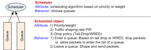
Scheduler: schedules multiple queues. The scheduler performs a specific scheduling algorithm to determine the order in which packets are forwarded. The scheduling algorithm can be Strict Priority (SP) or weight-based scheduling. The weight-based scheduling algorithms include Deficit Round Robin (DRR), Weighted Round Robin (WRR), Deficit Weighted Round Robin (WDRR), and Weighted Fair Queuing (WFQ). For details about scheduling algorithms, see Queues and Congestion Management.

The scheduler performs one action: selecting a queue. After a queue is selected by a scheduler, the packets in the front of the queue are forwarded.
Scheduled object: refers to a queue. Packets are sequenced in queues in the buffer.

Three configurable attributes are delivered to a queue:

(1) Priority or weight

(2) PIR

(3) Drop policy, including tail drop and Weighted Random Early Detection (WRED)

Packets may enter or leave a queue:

(1) Entering a queue: The device determines whether to drop a received packet based on the drop policy. If the packet is not dropped, it enters the tail of the queue.

(2) Leaving a queue: After a queue is selected by a scheduler, the packets in the front of the queue are shaped and then forwarded out of the queue.

Hierarchical Scheduling Model

HQoS uses a tree-shaped hierarchical scheduling model. As shown in Figure 1, the hierarchical scheduling model consists of three types of nodes:

Leaf node: is located at the bottom layer and identifies a queue. The leaf node is a scheduled object and can only be scheduled.
Transit node: is located at the medium layer and refers to both a scheduler and a scheduled object. When a transit node functions as a scheduled object, the transit node can be considered a virtual queue, which is only a layer in the scheduling architecture but not an actual queue that consumes buffers.
Root node: is located at the top layer and identifies the top-level scheduler. The root node is only a scheduler but not a scheduled object. The PIR is delivered to the root node to restrict the output bandwidth.

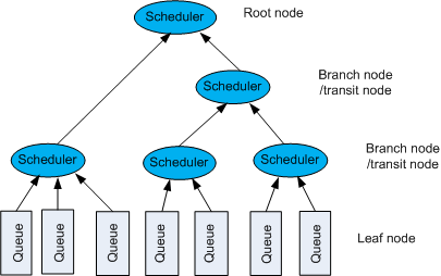
Figure 1 Hierarchical scheduling model

A scheduler can schedule multiple queues or schedulers. The scheduler can be considered a parent node, and the scheduled queue or scheduler can be considered a child node. The parent node is the traffic aggregation point of multiple child nodes.

Traffic classification rules and control parameters can be specified on each node to classify and control traffic. Traffic classification rules based on different user or service requirements can be configured on nodes at different layers. In addition, different control actions can be performed for traffic on different nodes. This ensures multi-layer/user/service traffic management.

HQoS Hierarchies

In HQoS scheduling, one-layer transit node can be used to implement three-layer scheduling architecture, or multi-layer transit nodes can be used to implement multi-layer scheduling architecture. In addition, two or more hierarchical scheduling models can be used together by mapping a packet output from a scheduling model to a leaf node in another scheduling model, as shown in Figure 2. This provides flexible scheduling options.

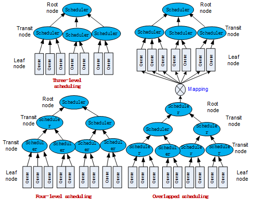
Figure 2 Flexible HQoS hierarchies

HQoS hierarchies supported by devices of different vendors may be different.

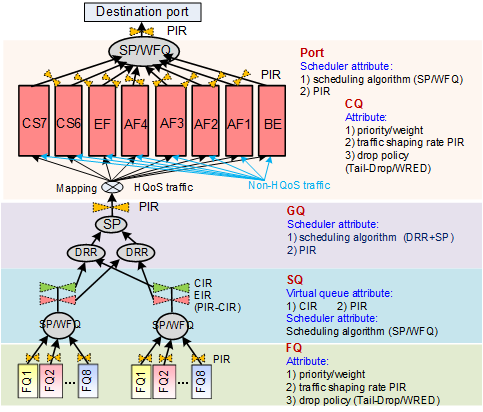
Scheduling Architecture of NetEngine 8000 Fs

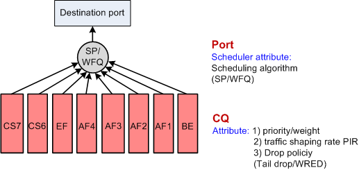
Figure 3 shows class queues (CQs) and port schedulers. NetEngine 8000 Fs not configured with HQoS have only CQs and port schedulers.

Figure 3 Scheduling architecture without HQoS

As shown in Figure 4, when HQoS is configured, a router specifies a buffer for flow queues that require hierarchical scheduling and performs a round of multi-layer scheduling for these flow queues. After that, the router puts HQoS traffic and non-HQoS traffic together into the CQ for unified scheduling.

Figure 4 HQoS scheduling
Click to enlarge

Leaf node: flow queue (FQ)

A leaf node is used to buffer data flows of one priority for a user. Data flows of each user can be classified into one to eight priorities. Each user can use one to eight FQs. Different users cannot share FQs. A traffic shaping value can be configured for each FQ to restrict the maximum bandwidth.

FQs and CQs share the following configurable attributes:
- Queue priority and weight
- PIR
- Drop policy, including tail drop and WRED
Transit node: subscriber queue

An SQ indicates a user (for example, a VLAN, LSP, or PVC). You can configure the CIR and PIR for each SQ.

Each SQ corresponds to eight FQ priorities, and one to eight FQs can be configured. If an FQ is idle, other FQs can consume the bandwidth of the FQ, but the bandwidth that can be used by an FQ cannot exceed the PIR of the FQ.

An SQ functions as both a scheduler and a virtual queue to be scheduled.
- As a scheduler: schedules multiple FQs. Priority queuing (PQ), Weighted Fair Queuing (WFQ), or low priority queuing (LPQ) applies to an FQ. The FQs with the service class EF, CS6, and CS7 use SP scheduling by default. The flow queues with the service class BE, AF1, AF2, AF3, and AF4 use WFQ scheduling by default, with the weight 10:10:10:15:15.
- As a virtual queue to be scheduled: is allocated two attributes, CIR and PIR. Using metering, the SQ traffic is divided into two parts, the part within the CIR and the burst part within the PIR. The former part is paid by users, and the latter part is also called the excess information rate (EIR). The EIR can be calculated using this format: EIR = PIR - CIR. The EIR refers to the burst traffic rate, which can reach a maximum of PIR.
- Root node: group queue (GQ)
  
  To simplify operation, you can define multiple users as a GQ, which is similar to a BGP peer group that comprises multiple BGP peers. For example, all users that require the same bandwidth or all premium users can be configured as a GQ.
  
  A GQ can be bound to multiple SQs, but an SQ can be bound only to one GQ.
  
  A GQ schedules SQs. DRR is used to schedule the traffic within CIR between SQs. If any bandwidth is remaining after the first round, DRR is used to schedule the EIR traffic. The bandwidth of CIR is preferentially provided, and the burst traffic exceeded the PIR is dropped. Therefore, if the bandwidth of a GQ reaches the PIR, the CIR of each SQ in the GQ can be guaranteed, and the maximum bandwidth that each SQ can obtain is its own PIR.
  
  In addition, a GQ, as a root node, can be configured with a PIR attribute to restrict the sum rate of multiple member users of the GQ. All users in this GQ are restricted by the PIR. The PIR of a GQ is used for rate limit but does not provide bandwidth guarantee. The PIR of a GQ is recommended to be greater than the sum of CIRs of all its member SQs. Otherwise, a user (SQ) cannot obtain sufficient bandwidth.
The following example illustrates the relationship between an FQ, SQ, and GQ.

In an example, 20 residential users live in a building. Each residential user purchases the bandwidth of 20 Mbit/s. To guarantee the bandwidth, an SQ with both the CIR and PIR of 20 Mbit/s is created for each residential user. The PIR here also restricts the maximum bandwidth for each residential user. With the subscription of VoIP and IPTV services as well as the HSI services, carriers promote a new bandwidth package with the value-added services (including VoIP and IPTV) added but the bandwidth 20 Mbit/s unchanged. Each residential user can use VoIP, IPTV, and HSI services.

To meet such bandwidth requirements, HQoS is configured as follows:
- Configure three FQs, corresponding to three services (VoIP, IPTV, and HSI), and set a CIR and PIR for each service.
- Altogether 20 SQs are configured for 20 residential users. The CIR and PIR are configured for each SQ.
- One GQ is configured for the whole building and corresponds to 20 residential users. The sum bandwidth of the 20 residential users is actually the PIR of the GQ. Each of the 20 residential users uses services individually, but the sum bandwidth of them is restricted by the PIR of the GQ.
The hierarchy model is as follows:
- FQs are used to distinguish services of a user and control bandwidth allocation among services.
- SQs are used to distinguish users and restrict the bandwidth of each user.
- GQs are used to distinguish user groups and control the traffic rate of twenty SQs.
FQs enable bandwidth allocation among services. SQs distinguish each user. GQs enable the CIR of each user to be guaranteed and all member users to share the bandwidth.

The bandwidth exceeds the CIR is not guaranteed because it is not paid by users. The CIR must be guaranteed because the CIR has been purchased by users. As shown in Figure 4, the CIR of users is marked, and the bandwidth is preferentially allocated to guarantee the CIR. Therefore, the bandwidth of CIR will not be preempted by the burst traffic exceeded the service rates.

On NetEngine 8000 Fs, HQoS uses different architectures to schedule upstream or downstream queues.

CAR-based HQoS

This function applies only to incoming traffic of user queues. The application scenario is the same as that of common HQoS.

This function is implemented by replacing FQ queues with CAR token buckets. The scheduling at other layers is the same as that of common HQoS. In this case, the forwarding module notifies the eTM module of the status of the token bucket, and then the eTM module adds tokens and determines whether to discard or forward the packets.

HQoS Scheduling for Downstream Queues

Figure 5 TM Scheduling architecture for downstream queues

Downstream TM scheduling includes the scheduling paths FQ -> SQ -> GQ and CQ -> port. There are eight CQs for downstream traffic, CS7, CS6, EF, AF4, AF3, AF2, AF1, and BE. Users can modify the queue parameters and scheduling parameters.

The process of downstream TM scheduling is as follows:

Entering a queue: An HQoS packet enters an FQ.
Applying for scheduling: The downstream scheduling application path is (FQ -> SQ -> GQ) + (GQ -> destination port).
Hierarchical scheduling: The downstream scheduling path is (destination port -> CQ) + (GQ -> SQ -> FQ).
Leaving a queue: After an FQ is selected, packets in the front of the FQ leave the queue and enters the CQ tail. The CQ forwards the packet to the destination port.

Non-HQoS traffic directly enters eight downstream CQs, without passing FQs.

**Table 1** Parameters for downstream TM scheduling
Queue/Scheduler	Queue Attribute	Scheduler Attribute
FQ	Queue priority and weight, which can be configured. PIR, which can be configured. The PIR is not configured by default. Drop policy, which can be configured as WRED. The drop policy is tail drop by default.	-
SQ	CIR, which can be configured. PIR, which can be configured.	To be configured. PQ and WFQ apply to FQs. By default, PQ applies to EF, CS6, and CS7 services; WFQ applies to BE, AF1, AF2, AF3 and AF4 services.
GQ	PIR, which can be configured. The PIR is used to restrict the bandwidth but does not provide any bandwidth guarantee.	Not to be configured. DRR is used to schedule the traffic within CIR between SQs. If any bandwidth is remaining after the first round, DRR is used to schedule the EIR traffic. The bandwidth of CIR is preferentially provided, and the burst traffic exceeded the PIR is dropped.
CQ	Queue priority and weight, which can be configured. PIR, which can be configured. The PIR is not configured by default. Drop policy, which can be configured as WRED. The drop policy is tail drop by default.	-
Port	PIR, which can be configured.	To be configured. PQ and WFQ apply to FQs. By default, PQ applies to EF, CS6, and CS7 services; WFQ applies to BE, AF1, AF2, AF3 and AF4 services.

Downstream scheduling

Figure 6 scheduling architecture for downstream queues
Click to enlarge

Unlike downstream TM scheduling, downstream scheduling is a five-level scheduling architecture. Downstream scheduling uses only FQs but not CQs. In addition to the scheduling path FQ -> SQ -> GQ, a parent GQ scheduling, also called a virtual interface (VI) scheduling, is implemented.

The VI is only a name of a scheduler but not a real virtual interface. In actual applications, a VI corresponds to a sub-interface or a physical interface. The VI refers to different objects in different applications.

The differences between downstream TM scheduling and downstream eTM scheduling are as follows:

Downstream TM scheduling uses two scheduling architectures. The five-level scheduling consists of two parts, (FQ -> SQ -> GQ) + (CQ -> port). HQoS traffic is scheduled in the path of FQ -> SQ -> GQ, and enters a CQ with non-HQoS traffic in the scheduling path of CQ -> port.
Downstream eTM, an entity queue scheduling method, uses the scheduling path of FQ -> SQ -> GQ -> VI -> port. The system sets a default SQ for eight CQs configured for non-HQoS traffic. The SQ directly participates in the port scheduling.

**Table 2** Parameters for downstream scheduling
Queue/Scheduler	Queue Attribute	Scheduler Attribute
FQ	Queue priority and weight, which can be configured. PIR, which can be configured. The PIR is not configured by default. Drop policy, which can be configured as WRED. The drop policy is tail drop by default.	-
SQ	CIR, which can be configured. PIR, which can be configured.	To be configured. PQ and WFQ apply to FQs. By default, PQ applies to EF, CS6, and CS7 services; WFQ applies to BE, AF1, AF2, AF3 and AF4 services.
GQ	PIR, which can be configured. The PIR is used to restrict the bandwidth but does not provide any bandwidth guarantee.	Not to be configured. DRR is used to schedule the traffic within CIR between SQs. If any bandwidth is remaining after the first round, DRR is used to schedule the EIR traffic. The bandwidth of CIR is preferentially provided, and the burst traffic exceeded the PIR is dropped.
Parent GQ/VI	PIR, which can be configured. The PIR is used to restrict the bandwidth but does not provide any bandwidth guarantee.	Different scheduling algorithms, such as DRR and WFQ, are used on different boards.
Port	PIR, which can be configured.	To be configured. PQ and WFQ apply to FQs. By default, PQ applies to EF, CS6, and CS7 services; WFQ applies to BE, AF1, AF2, AF3 and AF4 services.

Difference Between Downstream TM Scheduling and eTM Scheduling

**Table 3** Difference between downstream TM scheduling and eTM scheduling
Difference	Downstream TM Scheduling	Downstream eTM Scheduling
port-queue command	This command takes effect for traffic of a specific priority on an interface.	This command takes effect for traffic of a specific priority in a non-flow queue.
GQ bandwidth share	The GQ bandwidth can be shared by its member SQs on a TM module if the same GQ profile is used.	The GQ bandwidth can be shared by its member SQs only on the same interface, even if the same GQ profile is used.
SQ bandwidth share	Multiple SQs in the same GQ on different physical interfaces share the bandwidth.	Multiple SQs in the same GQ on different sub-interfaces but not physical interfaces share the bandwidth.
Trunk and member interfaces	The port-queue command can be configured on a trunk interface or its member interfaces. The command configuration on a member interface takes effect preferentially and schedules all traffic on the member interface.	The port-queue command can be configured on a trunk interface or its member interfaces, but the command configuration takes effect only for non-flow queues.

Use traffic shaping as an example to illustrate the difference between downstream TM scheduling and eTM scheduling. Assume that traffic shaping is configured for port queues on an interface and for flow queues or user queues on a sub-interface.

flow-queue FQ
  queue ef shaping 10M

interface gigabitethernet0/1/0
  port-queue ef shaping 100M

interface gigabitethernet0/1/0.1
  user-queue cir 50m pir 50m flow-queue FQ

interface gigabitethernet0/1/0.2
   //Note: user-queue and qos-profile are not configured on gigabitethernet0/1/0.2.

For downstream TM scheduling, the traffic shaping rate configured using the port-queue command determines the sum bandwidth of both HQoS and non-HQoS traffic. Based on the preceding configuration:
- The rate of EF traffic sent from GE 0/1/0.1 does not exceed 10 Mbit/s.
- The rate of EF traffic sent from GE 0/1/0 (including GE 0/1/0, GE 0/1/0.1, and GE 0/1/0.2) does not exceed 100 Mbit/s.
For downstream eTM scheduling, the traffic shaping rate configured using the port-queue command determines the sum bandwidth of non-HQoS traffic (default SQ bandwidth). Based on the preceding configuration:
- The rate of EF traffic sent from GE 0/1/0 and GE 0/1/0.2 (non-HQoS traffic) does not exceed 100 Mbit/s.
- The rate of EF traffic sent from GE 0/1/0.1 does not exceed 10 Mbit/s.
- The rate of EF traffic sent from GE 0/1/0 can reach a maximum of 110 Mbit/s.

HQoS Scheduling Tree Split on a Trunk Interface

When traffic on a trunk interface is scheduled using HQoS based on the TM, if a trunk member interface is congested, traffic on other member interfaces is affected. After the HQoS scheduling tree on a trunk interface is split, a scheduling tree is created based on each trunk member interface. HQoS scheduling can be performed for traffic on a trunk interface based on the trunk member interfaces.

When three interfaces of one TM are added to a trunk interface, the HQoS scheduling tree of the trunk interface is as follows:

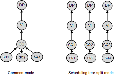
Figure 7 HQoS scheduling tree model of a trunk interface

When HQoS is used, HQoS needs to apply for bandwidth based on a trunk's member interfaces. Each member interface applies for a resource and performs HQoS scheduling independently.

HQoS Priority Mapping

Both upstream HQoS scheduling and downstream HQoS scheduling use two entity queues: eight FQs and four CQs for upstream scheduling, and eight FQs and eight CQs for downstream scheduling. Packets enter an FQ based on the service class. After that, packets in the front of the FQ queue leave the queue and enter a CQ based on the mapping.

The mapping from FQs to CQs can be in Uniform or Pipe mode.

Uniform: The system defines a fixed mapping. Upstream scheduling uses the uniform mode.
Pipe: Users can modify the mapping. The original priorities carried in packets will not be modified in pipe mode.

By default, in the downstream HQoS, the eight priority queues of an FQ and eight CQs are in one-to-one mapping. In the upstream HQoS, COS0 corresponds to CS7, CS6, and EF, COS1 corresponds to AF4 and AF3, COS2 corresponds to AF2 and AF1, and COS3 corresponds to BE.

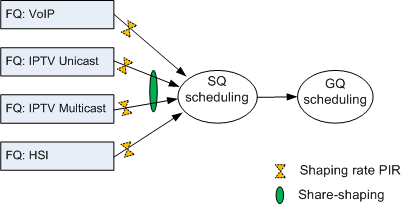
Share Shaping

Share shaping, also called Flow Group Queue shaping (FGQ shaping), implements traffic shaping for a group that two or more flow queues (FQs) in a subscriber queue (SQ) constitute. This ensures that other services in the SQ can obtain bandwidths.

For example, a user has HSI, IPTV, and VoIP services, and IPTV services include IPTV unicast and multicast services. To ensure the CIR of IPTV services and prevent IPTV services from preempting the bandwidth reserved for HSI and VoIP services, you can configure four FQs, each of which is specially used for HSI, IPTV unicast, and IPTV multicast, and VoIP services. As shown in Figure 8, share shaping is implemented for IPTV unicast and multicast services, and then HQoS is implemented for all services.

Figure 8 Share shaping

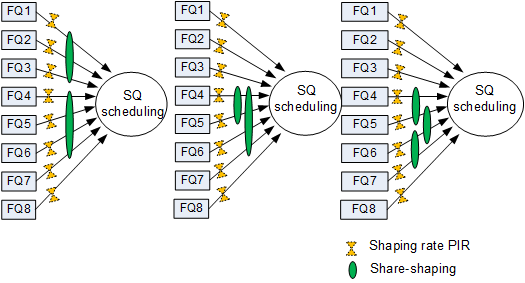
Currently, a maximum of two share shaping configurations can be configured for eight FQs on each SQ, as shown by the first two modes in Figure 9. The third share shaping mode shown in Figure 9 is not available on the NetEngine 8000 F.

Figure 9 Share shaping modes on a NetEngine 8000 F

Share shaping can be implemented in either of the following modes on a NetEngine 8000 F:

Mode A: Share shaping only shapes but not schedule traffic, and queues to which share shaping applies can use different scheduling algorithms.
Mode B: Queues to which share shaping applies must share the same scheduling algorithm. These share-shaping-capable queues are scheduled in advance, and then scheduled with other queues in the SQ as a whole. When share-shaping-capable queues are scheduled with other queues in the SQ, the highest priority of the share-shaping-capable queues becomes the priority of the share-shaping-capable queues as a whole, and the sum of weights of the share-shaping-capable queues become the weight of the share-shaping-capable queues as a whole.

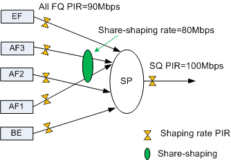
Example 1: As shown in Figure 10, the traffic shaping rate of the BE, EF, AF1, AF2, and AF3 queues is 90 Mbit/s, and the sum bandwidth of the SQ is 100 Mbit/s. All queues use the strict priority (SP) scheduling. After share shaping is configured, the sum bandwidth of the AF1 and AF3 queues is set to 80 Mbit/s.

Figure 10 SP scheduling for share shaping

Assume that the PIR is ensured for the SQ. The input rate of the EF queue is 10 Mbit/s, and that of each other queue is 70 Mbit/s. Share shaping allocates bandwidths to the queues in either of the following modes:

Mode A: SP scheduling applies to all queues.
- The EF queue obtains the 10 Mbit/s bandwidth, and the remaining bandwidth is 90 Mbit/s.
- The bandwidth allocated to the AF3 queue is calculated in the following format: Min { AF3 PIR, share-shaping PIR, SQ PIR, remaining bandwidth} = Min {90 Mbit/s, 80 Mbit/s, 100 Mbit/s, 90 Mbit/s} = 80 Mbit/s. The traffic rate of the AF3 queue, however, is only 70 Mbit/s. Therefore, the AF3 queue actually obtains the 70 Mbit/s bandwidth, leaving the 20 Mbit/s bandwidth available for other queues.
- The bandwidth allocated to the AF2 queue is calculated in the following format: Min { AF2 PIR, SQ PIR, remaining bandwidth}= Min {90 Mbit/s, 100 Mbit/s, 20 Mbit/s} = 20 Mbit/s. Therefore, the AF2 queue obtains the 20 Mbit/s bandwidth, and no bandwidth is remaining.
- The AF1 and BE queues obtain no bandwidth.
Mode B: The EF is scheduled first, and then AF3 and AF1 are scheduled as a whole, and then BE is scheduled.
- The EF queue obtains the 10 Mbit/s bandwidth, and the remaining bandwidth is 90 Mbit/s.
- The bandwidth allocated to the AF3 queue is calculated in the following format: Min { AF3 PIR, share-shaping PIR, SQ PIR, remaining bandwidth} = Min {90 Mbit/s, 80 Mbit/s, 100 Mbit/s, 90 Mbit/s} = 80 Mbit/s. The input rate of the AF3 queue, however, is only 70 Mbit/s. Therefore, the AF3 queue actually obtains the 70 Mbit/s bandwidth, leaving the 20 Mbit/s bandwidth available for other queues.
- The bandwidth allocated to the AF2 queue is calculated in the following format: Min { AF1 PIR, share-shaping PIR - AF3 bandwidth, SQ PIR, remaining bandwidth } = Min {90 Mbit/s, 10 Mbit/s, 20 Mbit/s} = 10 Mbit/s. Therefore, the AF1 queue obtains the 10 Mbit/s bandwidth, and the remaining bandwidth becomes 10 Mbit/s.
- The bandwidth allocated to the AF2 queue is calculated in the following format: Min { AF2 PIR, SQ PIR, remaining bandwidth } = Min { 90 Mbit/s, 100 Mbit/s, 10 Mbit/s } = 10 Mbit/s. Therefore, the AF2 queue obtains the 10 Mbit/s bandwidth, and no bandwidth is remaining.
- The BE queue obtains no bandwidth.
The following table shows the bandwidth allocation results.

Queue	Scheduling Algorithms	Input Bandwidth (Mbit/s)	PIR (Mbit/s)	Output Bandwidth (Mbit/s)
Queue	Scheduling Algorithms	Input Bandwidth (Mbit/s)	PIR (Mbit/s)	Mode A	Mode B
EF	SP	10	90	10	10
AF3	SP	70	90	70	70
AF2	SP	70	90	20	10
AF1	SP	70	90	0	10
BE	SP	70	Not configured	0	0

Example 2: Assume that the WFQ scheduling applies to the EF, AF1, AF2, and AF3 queues with the weight ratio as 1:1:1:2 (EF:AF3:AF2:AF1) in example 1. The LPQ scheduling applies to the BE queue. The PIR 100 Mbit/s is ensured for the SQ. The input rate of the EF and AF3 queues is 10 Mbit/s, and that of each other queue is 70 Mbit/s. Share shaping allocates bandwidths to the queues in either of the following modes:

Mode A: The WFQ scheduling applies to all queues.

First-round WFQ scheduling:
- The bandwidth allocated to the EF queue is calculated as follows: 1/(1 + 1 + 1 + 2) x 100 Mbit/s=20 Mbit/s. The input rate of the EF queue, however, is only 10 Mbit/s. Therefore, the remaining bandwidth is 90 Mbit/s.
- The bandwidth allocated to the AF3 queue is calculated as follows: 1/(1 + 1 + 1 + 2) x 100 Mbit/s=20 Mbit/s. The input rate of the AF3 queue, however, is only 10 Mbit/s. Therefore, the remaining bandwidth is 80 Mbit/s.
- The bandwidth allocated to the AF2 queue is calculated as follows: 1/(1 + 1 + 1 + 2) x 100 Mbit/s=20 Mbit/s. Therefore, the AF2 queue obtains the 20 Mbit/s bandwidth, and the remaining bandwidth becomes 60 Mbit/s.
- The bandwidth allocated to the AF1 queue is calculated as follows: 2/(1 + 1 + 1 + 2) x 100 Mbit/s=40 Mbit/s. Therefore, the AF2 queue obtains the 40 Mbit/s bandwidth, and the remaining bandwidth becomes 20 Mbit/s.
Second-round WFQ scheduling:
- The bandwidth allocated to the AF2 queue is calculated as follows: 1/(1 + 2) x 20 Mbit/s = 6.7 Mbit/s.
- The bandwidth allocated to the AF1 queue is calculated as follows: 2/(1 + 2) x 20 Mbit/s = 13.3 Mbit/s.
No bandwidth is remaining, and the BE queue obtains no bandwidth.

Mode B: The AF3 and AF1 queues, as a whole, are scheduled with the EF and AF2 queues using the WFQ scheduling. The weight ratio is calculated as follows: EF:(AF3+AF1):AF2 = 1:(1+2):1 = 1:3:1.

First-round WFQ scheduling:

The bandwidth allocated to the EF queue is calculated as follows: 1/(1 +3 + 1) x 100 Mbit/s=20 Mbit/s. The input rate of the EF queue, however, is only 10 Mbit/s. Therefore, the EF queue actually obtains the 10 Mbit/s bandwidth, and the remaining bandwidth is 90 Mbit/s.
The bandwidth allocated to the AF3 and AF1 queues, as a whole, is calculated as follows: 3/(1 + 3 + 1) x 100 Mbit/s = 60 Mbit/s. Therefore, the remaining bandwidth becomes 30 Mbit/s. The 60 Mbit/s bandwidth allocated to the AF3 and AF1 queues as a whole are further allocated to each in the ratio of 1:2. The 20 Mbit/s bandwidth is allocated to the AF3 queue. The input rate of the AF3 queue, however, is only 10 Mbit/s. Therefore, the AF3 queue actually obtains the 10 Mbit/s bandwidth, and the remaining 50 Mbit/s bandwidth is allocated to the AF1 queue.
The bandwidth allocated to the AF2 queue is calculated as follows: 1/(1 +3 + 1) x 100 Mbit/s=20 Mbit/s. Therefore, the AF2 queue obtains the 20 Mbit/s bandwidth, and the remaining bandwidth becomes 10 Mbit/s.

Second-round WFQ scheduling:

The bandwidth allocated to the AF3 and AF1 queues as a whole is calculated as follows: 3/(3 + 1) x 10 Mbit/s=7.5 Mbit/s. The 7.5 Mbit/s bandwidth, not exceeding the share shaping bandwidth, can be all allocated to the AF3 and AF1 queues as a whole. The PIR of the AF3 queue has been ensured. Therefore, the 7.5 Mbit/s bandwidth is allocated to the AF1 queue.
The bandwidth allocated to the AF2 queue is calculated as follows: 1/(3 + 1) x 10 Mbit/s = 2.5 Mbit/s.

No bandwidth is remaining, and the BE queue obtains no bandwidth.

The following table shows the bandwidth allocation results.

Queue	Scheduling Algorithms	Input Bandwidth (Mbit/s)	PIR (Mbit/s)	Output Bandwidth (Mbit/s)
Queue	Scheduling Algorithms	Input Bandwidth (Mbit/s)	PIR (Mbit/s)	Mode A	Mode B
EF	SP	10	90	10	10
AF3	SP	70	90	10	70
AF2	SP	70	90	26.7	22.5
AF1	SP	70	90	53.3	57.5
BE	SP	70	Not configured	0	0